

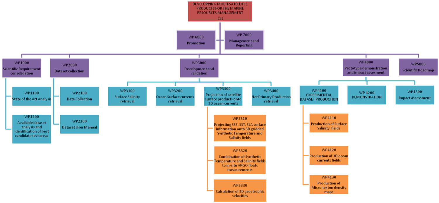
Project Workpackage Breakdown Structure
WP1000: Scientific Requirements
Consolidation
WP2000: Dataset collection
WP3000: Development and validation
WP4000: Prototype demonstration and impact assessment
WP5000: Scientific Roadmap
WP6000: Promotion
WP7000: Management and Reporting
WP1000: Scientific Requirements Consolidation
The theme investigated in this project is the unique synergetic capability of past and present ESA and non-ESA Earth Observation mission to provide the required multi-missions products to be used as inputs to a micronekton model in order to produce maps of distribution of biomass of several micronekton functional groups. Three key variables are needed as forcing to the micronekton model: the Temperature, the ocean currents and the primary production. In this workpackage, we will consolidate the scientific requirements regarding these three variables. In particular, the production of 3D ocean currents products from the synergetic use of altimetry, gravity, satellite Sea Surface Salinity, and satellite Sea Surface Temperature.
WP1100: State of the Art Analysis
We will perform a
detailed review of the existing multi-mission Sea
Surface Temperature, Sea Surface Salinity and Sea Surface Height
products, together with the existing methodologies aiming at merging
this information and project it from the surface to depth in order to
produce 3D maps of ocean currents. We will also review the existing Net
Primary Production products available from the processing of space-born
ocean color measurements (together with SST and solar radiation).
All available products will be analyzed focussing on their major
limitations and drawbacks in relation to their use as forcing products
for micronekton modelling.
This review will include a survey of current and upcoming initiatives
related to the project.
WP1200 Available dataset analysis and identification of best candidate test areas
In order to identify the best candidate test areas to be used in the following tasks for development and validation of the prototype products, we will perform a detailed review of all space-borne and in-situ datasets available for the subsequent development and validation tasks. Together with the availability and accuracy of data, the identification of the best candidate test areas will also be strongly based on the a-priori knowledge of the interesting test areas from the point of view of marine resource management. A preliminary list of potential test areas is given in section 2.6.
These two subtasks will lead to issuing a consolidated risk analysis together with a consolidated, coherent and complete view of the scientific and operational requirements associated with the management of marine resources from multimissions products.
Output:
As output, a Requirement Baseline (RB) document will be issued, that
will include a complete and detailed description of the information
requirements concerning the calculation of ocean 3D currents from the
merging of space-born measurements for the modeling of micronekton
density.
WP2000: Dataset collection
WP2100: Data collection
In this task, a
database of suitable EO based products, in situ
data and relevant ancillary information will be collected over the
areas of interest. This will include all data needed for the
calculation of the improved surface salinity products, the calculation
of the observed 3D ocean surface currents, as well as the data needed
as input to the micronekton model (primary production) and all data
needed for validation purposes (in-situ acoustic measurements of
micronekton density). The database will be made accessible on the
project webpage.
Any restrictions in the use of any type of datasets (e.g., proprietary
campaign data) will be communicated to ESA in due time.
A first list of required data is provided in section 2.5 (Data
Procurement Plan). They include all the ESA Earth Explorer satellite
data mentioned in the Statement of Work: SMOS, Cryosat and GOCE,
together with other ESA and non ESA satellite measurements archive, and
in-situ data.
WP2200: Dataset User Manual
In this task, a Data User Manual will be written, that will contain a detailed description of the dataset as well as the related metadata.
Output:
The following outputs will be delivered as required:
- Dataset
- Dataset User Manual
WP3000: Development and validation
In this work package, we will perform the required R&D activities needed for the Prototype Demonstration Work Package. The time periods and test areas where this work will be done, together with the required spatial and temporal resolution of the target final products will be defined in details at the beginning of the project thanks to the outputs from the WP1000 and WP2000. However, first plans are to focus our test areas in the tropical and southern Pacific Ocean and the Indian Ocean Austral region where collaborations with colleagues from CSIRO Australia, NOAA-Hawaii and CNRS/IRD France are on-going (see also section 2.6). The output resolution will be 1/4°x week and may be increased to 1/12°x day in some specific region (e.g. Kerguelen Islands area) for specific validation studies.
WP3100: Surface Salinity retrieval from SMOS, SST and Argo data
The interpolation
method proposed here to merge SMOS and in situ
SSS measurements and build a high resolution SSS L4 product consists of
a four-dimensional version of the Optimal Interpolation (OI) technique
(Bretherton & al., 1976). It has been first developed and tested by
Buongiorno Nardelli (2012) on the North Atlantic, and successively used
also for other areas (e.g. Buongiorno Nardelli, 2013). The methodology
maximizes the synergy between different sensors by taking advantage of
the correlation between SSS and high-pass filtered SST measurements,
thus allowing to increase the effective SSS resolution (up to 1/10° x
1/10°, daily) by extracting small scale patterns from high resolution
satellite estimates of the SST. A similar (though simpler) technique,
based on local weighted regressions between satellite SSS and SST, has
recently been applied to SMOS measurements by Umbert & al. (2013).
In fact, in the classical formulation of the Optimal Interpolation (OI)
technique, as well as in many successive applications (e.g., Gouretski
and Koltermann 2004), the covariance function used is estimated from a
functional fit of the autocorrelation of the observations as a function
of distance, and the field to be interpolated is defined in a
bi-dimensional Euclidean space [i.e., the geographical space (x,y)].The
distance is thus simply given by the spatial separation. However, OI
theory remains valid also considering other Euclidean spaces, provided
suitable ''generalized'' distance and covariance models are defined. A
typical example is the inclusion of the 'time' variable, (x, y, t), so
that observations collected within a temporal window close to the
interpolation point can be more efficiently combined to improve the
estimate, taking into account the temporal correlation of the field
(e.g., Le Traon & al. 1998; Charraudeau and Gaillard 2007).
At the oceanic mesoscale, i.e. (10 - 100 km), and smaller scales, (<
10 km), one of the assumptions of the standard OI algorithm,
statistical stationarity, is likely to fail, and the choice of a fixed
covariance model based only on space and time separation may not be
optimal. For example, SSS covariance is expected to be spatially
anisotropic and nonstationary in frontal areas and in regions
characterized by strong mesoscale activity. Actually, small spatial
decorrelation scales will be found perpendicular to the isothermals
(because density differences are generally due to the presence of water
masses characterized by different T and S values) rather than along the
isothermals (where differences are basically due to isopycnal mixing
alone). On the other hand, the decorrelation scales would certainly be
modified locally by the field evolution/displacement.
As shown in Buongiorno Nardelli (2012), one way to account for part of
this nonstationarity is to represent SSS as a function of space, time,
and high-pass filtered SST (fSST) or, in other words, to define the
variable to be interpolated in the four-dimensional space (x, y, t,
fSST). A new stationary covariance model is thus defined by including a
thermal decorrelation term. This particular covariance model allows to
give a higher weight to the SSS observations that lie on the isothermal
of the interpolation point with respect to observations taken at the
same temporal and spatial separation but characterized by different SST
values. This technique has been already applied to interpolate SSS ARGO
measurements at 1/10° x 1/10°, daily resolution, using GHRSST L4 SST
data to compute the covariances.
In this project, the four-dimensional OI technique briefly described
above will be adapted to ingest SMOS (end eventually AQUARIUS) L2
and/or L3 data, either as additional observations and/or to build a new
first guess field, concentrating on the test area/period selected. This
will require a specific analysis/interpretation of the errors
associated with SMOS products (starting from most recent results
published on the matter, e.g. Boutin & al., 2012, 2013; Yin &
al., 2012, 2013; Font & al., 2013), in order to properly define the
observation error covariances for the OI (also keeping into account
representativeness differences between the various products).
Background errors and all other relevant parameters needed by the OI
will be derived through specific independent validation/tuning
exercises, starting from the approach followed in Buongiorno Nardelli
(2012).
As discussed in Buongiorno Nardelli (2012), the four-dimensional
covariance model is expected to provide more accurate results in the
open ocean than in coastal areas or semi-enclosed seas.
The task will thus require the following activities:
- analysis/interpretation of the errors associated with state-of-the-art SMOS products, also keeping into account the space-time representativeness of the various SSS products, in situ and satellite SST data, starting from an in depth analysis of the most recent literature and documentation available,
- identification of the OI configurations to be tested in terms of input data and first guess field definition, as well as of the spatial and temporal domains to be considered for the development and test,
- definition of the observation error covariances for each of the OI configurations to be tested; derivation of the corresponding background errors and of all other relevant parameters through specific independent validation/tuning exercises, basing on the approach followed by Buongiorno Nardelli (2012),
- comparison between the different test SSS L4 products; independent validation based on available thermosalinograph (TSG) data (for SSS) and hindcast validation by comparison with original ARGO surface measurements.
WP3200: Surface currents retrieval from GOCE and altimeter data
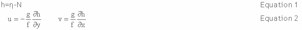
The GOCE (Gravity Field and Steady-State Ocean Circulation) satellite was successfully launched in March 2009. First Earth Explorer core mission from the ESA Living Planet program, its prime objective was to provide an estimate of the geoid's scales down to 100 km with centimetric accuracy [ESA, 1999] to serve the application of ocean circulation calculation. The geoid height N is indeed the missing quantity needed to compute (Equation 1) the ocean absolute dynamic topography (the sea level above the geoid) from the altimetric measurement (the sea level above a reference ellipsoid). Under geostrophic assumption, ocean surface currents can then be derived from the absolute dynamic topography (Equation 2).
In practice, the absolute dynamic topography cannot be computed as the simple difference between the altimetric measurement and the geoid height, as this would require to know the geoid with centimetric accuracy at scales down to a few hundred meters.
An altimeter provides indeed one sea level height measurement roughly every 350 m along-track, which are commonly averaged over 7 km in order to reduce noise. Alternatively, Sea Level Anomalies relative to a given time period P are computed using the repeat-track-method [Cheney & al, 1983], in which along-track mean altimetric profiles are subtracted from the instantaneous altimetric heights. To reconstruct the full dynamical signal from the altimetric anomaly, an accurate estimate of the ocean Mean Dynamic Topography (MDT) for the time period P is needed. The most straightforward approach is to subtract a geoid model from an altimetric Mean Sea Surface (MSS) defined as the gridded mean profiles , after making sure that both surfaces are consistent, and notably that they are expressed relative to the same ellipsoid and tide system (all details are given in Hughes and Bingham [2008]). However, altimetric MSS resolve much shorter spatial scales (down to 10 - 20 km) than recent satellite-only (i.e. computed from space gravity data only) geoid models and, in order to match the spectral content of both surfaces, filtering is needed. This can be done using simple filters as Gaussian or Hamming (Tapley & al. [2003], Jayne [2006], Bingham & al. [2008]). In order to remove as much noise as possible while minimizing signal attenuation, more complex filters may be used. For example, Vianna & al [2007, 2010] developed an adaptative filter, based on principal components analysis techniques, while Bingham [2010] applied a nonlinear anisotropic diffusive filtering.
In this task we will adapt and tune the optimal filtering technique developed by Rio & al [2011] in which both errors on the MSS and the geoid are taken into account, together with an a-priori knowledge of the MDT covariance structure, in order to smooth the noisy short scales while preserving the sharp gradients.
Compared to the previous fourth release, that was based on the use of 2 years of reprocessed GOCE data, this last release will benefit from the lowering of the GOCE orbit during the last year of his mission from 255 km down to an extremely low altitude of 224 km, providing accurate measurements of the Earth gravity at scales even shorter than the initial mission's objectives (100 km). Together with an altimeter MSS, this last GOCE geoid version will enable us to calculate an updated satellite-only Mean Dynamic Topography, to be subsequently used to compute maps of absolute dynamic topography, and by finite differentiation, maps of surface geostrophic currents on the selected test areas.
The different
activities during this WP will include:
- accurate error analysis of the fifth release of the GOCE geoid model
- tuning of the optimal filter for the selected test areas
- validation of the obtained MDT through comparison to other existing solutions and in-situ data (as surface drifters).
Output:
Expected outcomes are:
- a better representation of the ocean Mean Dynamic Topography in the selected test areas.
WP3300: Projection of satellite surface products onto ocean currents
The methods use
hereafter have been developed by the CLS team
during the past ten years and has been implemented in real-time as part
of the European MyOcean project (http://www.myocean.eu/) as the
observation-based component of the Global Ocean Monitoring and
Forecasting Center. It relies on the combination of in situ
(temperature and salinity profiles, surface drifting buoys) and
satellite observations (GOCE, altimetry, sea surface temperature)
through statistical methods. Global temperature and salinity (Guinehut
& al., 2012), absolute height and geostrophic current fields (Mulet
& al., 2012) are provided at weekly and monthly periods from the
surface down to 5500-meter depth and for the 1993-ongoing periods.
The objective of this workpackage is to improve the existing methods in
order to answer the scientific requirements listed in WP1000. This will
include the following three sub-workpackages.
WP 3310: Projecting SSS, SST, SLA surface information onto 3D gridded Synthetic Temperature and Salinity fields
The first step of the projection of satellite surface products onto ocean currents consists in deriving Synthetic temperature fields from satellite altimeter SLA and satellite SST observations using a multiple linear regression method. Synthetic salinity fields are also derived but, due to the lack in the past of satellite SSS, using a simple linear regression method of satellite altimeter SLA only. Covariances used in the linear regression methods have been computed from historical in situ observations and for the global ocean. They have been computed locally on a global 1° horizontal grid using all observations available in large radius of influence around each grid point (up to 5° in latitude and 25° in longitude) (see Guinehut & al., 2012).
In order to adapt the
method to the selected test area (see WP
1200) and to benefit from the surface salinity product retrieve in WP
3100, we thus propose here to:
- for the first time, use satellite SSS together with satellite altimeter SLA to reconstruct synthetic salinity fields at depth,
- calculate new regional covariances at higher horizontal and vertical resolution,
- validate the new synthetic temperature and salinity fields computed using independent in situ observations.
The first task will be
the evolution of the current method to
reconstruct synthetic salinity at depth from a simple linear regression
method of satellite altimeter SLA to a multiple linear regression
method of satellite altimeter SLA and the surface salinity fields
computed in WP 3100.
The proposed new method will require the computation of the covariances
between surface salinity and salinity at depth. All available in situ
observations collected in the selected test area (see WP 1200) will be
used to compute these covariances but also they will be used to improve
the current ones (between surface temperature and temperature at
depth). As the test area will probably be at basin scale, improved
resolution (horizontal and vertical) is required to better represent
the mix layer depth dynamics and also to better represent the vertical
projection of the mesoscale signals. Mix layer depth and mesoscale
dynamics are very important for micronekton dynamics. Several tests are
planned for the computation of the covariances in order to reduce
expected problems due to non-uniform temporal and spatial distribution
of in situ measurements. A compromise will have to be found between the
target resolution and the availability of the in situ observations.
Validation of synthetic temperature and salinity fields computed using
the new covariances and the new multiple linear regression methods
(SLA+SST for temperature, and SLA + SSS for salinity) will be performed
using independent in situ observations of temperature and salinity
profiles. Mean and rms of the differences between the two datasets (in
situ and synthetic) will be computed as a function of depth, time and
geographical areas.
Input data needed for this task are listed in the Data Procurement Plan
(section 2.5).
Output:
Expected outcomes are:
- a better representation of the mix layer depth dynamics,
- a better projection of the surface mesoscale signals onto depth,
- a better synthetic temperature and salinity fields reconstruction.
WP3320: Combination of Synthetic Temperature and Salinity fields to in-situ ARGO floats measurements
The second step of the
projection of satellite surface products
onto ocean currents consists in combining the synthetic estimates (WP
3310) with all available in situ temperature and salinity profiles
(Argo floats, XBTs, CTDs, moorings) using an optimal interpolation
method (Bretherton & al., 1976). The method was first developed
using simulated data (Guinehut & al., 2004) and is now applied to
real observations (Guinehut & al., 2012). The key issue is to gain
maximum benefit from the qualities of both datasets, namely the
accurate information given by the sparse in situ profiles and the
mesoscale content provided by the synthetic fields (deduced from
satellite observations). Le Traon & al. (1998) and Guinehut &
al. (2004) have shown that a precise statistical description of the
errors in these observations must be introduced in the optimal
interpolation method. In addition to the conventional use of a
measurement white noise representing 10 % of the signal variance, an a
priori bias of 20 % and a spatially correlated error of 20 % are also
applied to the synthetic fields to correct large-scale errors and bias
introduced by the first step of the method (i.e. the regression
method). The measurement white noise of 10 % of the signal variance
includes both instrument error (expected to be very small) and
representation error. Representation error, as defined by Oke and Sakov
(2008), is the component of observation error due to unresolved scales
and processes. In other words, it is the part of the true signal that
cannot be represented on the chosen grid due to limited spatial and
temporal resolution. As Oke and Sakov (2008) found values greater than
or comparable to measurement error in regions of strong mesoscale
variability, it is applied as a function of signal variance. As the
main objective of the combination is to correct the large-scale part of
the synthetic fields using the surrounding in situ profiles, signal
spatial correlation scales are set to twice those used to compute the
gridded altimeter maps (AVISO, 2012). They vary from 700 km (resp. 500
km) at the equator to 300 km north of 60°N in the zonal (resp.
meridional) directions. The temporal correlation scale is fixed at 15
days everywhere. The signal space-time correlation function is the same
as that used in Guinehut & al. (2004).
All the errors used in the current version of the method have been
estimated empirically and more accurate estimates are required to
optimally combine synthetic fields and in situ observations. Adapted
spatial and temporal correlation scales are also needed to better
represent the ocean dynamics in the selected test area (see WP 1200).
We thus propose here to:
- compute the errors associated to the synthetic fields,
- introduce these errors in the optimal interpolation method, and quantify their impact,
- test new temporal and spatial correlation scales in the optimal interpolation method, and quantify their impact
- validate the final combined temperature and salinity fields.
The optimal interpolation method requires indeed global error estimates (no gap), and relatively smooth temporal, horizontal and vertical structures.
Those newly estimated error will then be introduced in the optimal interpolation method. Their impact will be estimate in two ways. The first one will be a qualitative validation by visual inspection of the dynamical structures reconstructed. The second one will use Degree of Freedom of Signal (DFS) diagnostics for more quantitative estimates. DFS is an influence matrix diagnostics, first developed for the atmosphere (Cardinali & al., 2004), and now used for the ocean in data assimilation systems (Oke & al., 2009; Sakov & al., 2012) and also in the altimeter DUACS system (Dibarboure & al., 2011). It provides a measurement of the gain in information brought by the observations. DFS is calculated as the trace of the HK matrix, H being the observation operator and K the Kalman gain matrix. The optimal interpolation method used in the combination uses a Gauss-Markov estimator that provides a direct access to the HK matrix as it is explicitly computed along with the error covariance matrix or formal mapping error (Bretherton & al., 1976). DFS are computed on each HK matrix, meaning each grid point in case of a suboptimal optimal interpolation method. It is thus possible to use this metric to access the local mapping gain in information provided by each dataset (in situ, synthetic). Partial DFS are associated with a particular dataset and are computed from the partial trace of the HK matrix, taking only elements associated with the dataset to be analyzed. Partial DFS associated with the dataset i is written DFS(i). Two metrics will be particularly studied: (1) the fraction of the percentage of the overall information content (%IC) for in situ data and synthetic data (%IC = DFS(i)/ΣiDFS(i) x 100); and (2) the fraction of information of each data type actually exploited by the optimal interpolation system (%ICexploited = DFS(i)/N(i), where N(i) being the actual number of observations from dataset i; i.e., excluding information lost due to duplicate data). Those two metrics will help us to quantify where the information comes from in situ temperature and salinity profiles observations and where it comes from the synthetic fields. They will also help us to check whether information is redundant inside a specific dataset.
New temporal and spatial correlation scales will also be tested in the optimal interpolation method in order to better represent the ocean dynamics associated to the selected test area. As for the errors, impact of those correlation scales will be quantified using the same methods (visual inspection of the dynamical structures reconstructed and DFS diagnostics).
Validation of the combined temperature and salinity fields computed using the new errors and the new correlation scales will be performed using independent in situ observations of temperature and salinity profiles, if any, or using the in situ observations used in the combination method. The last validation is not independent but it nevertheless allows confirming than the merging method has been performed in an optimal way.
Input data needed for this task are listed in the Data Procurement Plan (section 2.5).
Output:
Expected outcomes are:
- a precise statistical description of the errors associated to the synthetic fields,
- a better representation of the temporal and spatial correlation scales in the selected test area,
- a better representation of the mix layer depth dynamics and of the mesoscale structures,
- a better combined temperature and salinity fields reconstruction.
WP3330: Calculation of 3D geostrophic velocities
The third step of the projection of satellite surface products onto ocean currents is based on the thermal wind equation (Equation 3) has been first investigated and described in Mulet & al (2013). It consists in combining the altimeter derived surface current estimates to 3D density fields using the thermal wind equation (Equation 3).
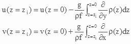
Equation 3
The reference level is
taken at the surface (z=0) where the
geostrophic currents are well known thanks to the combined use of GOCE
and altimetry, and have been tuned for the selected periods and test
areas in WP3200. The horizontal density gradient in the thermal wind
equation is computed from the thermohaline field calculated in WP3320.
A challenging issue when combining the surface geostrophic currents to
the 3D density field regards the respective spatial scale content of
the two fields (Mulet & al, 2013). Indeed, the two fields need to
resolve the same spatial scales if the surface information is to be
projected properly onto depth. For example, if the altimeter surface
currents resolve shorter scales than the density fields, short scales
surface information will be propagated all along the water column
resulting in a over barotropic velocity estimate of the ocean 3D
circulation.
This issue will be thoroughly and properly handled in this task in
order to produce the best possible 3D ocean current estimates over the
selected test areas. The spatial content of both the surface
geostrophic currents and the 3D thermohaline estimates will be
accurately analyzed and adequate filtering will be applied to ensure
consisteny between the two fields.
The obtained 3D ocean currents will be validated through comparison to
in-situ measurements of the ocean velocities (we will use for instance
the velocity estimates at 1 000 m depth derived from the displacement
of ARGO floats, as well as available currentmeter measurements), as
well as to outputs from ocean numerical models as the GLORYS2V3
reanalysis from the Mercator-Ocean system.
WP3400: Estimation of Net Primary Production from satellite Ocean Color data
In this task, maps of net primary production and associated euphotic layer will be calculated based on ocean color satellite data. Two different methods will be tested for the optimization experiences of the micronekton model: the VGPM and the CbPM models (more details on these two models are given on http://www.science.oregonstate.edu/ocean.productivity/index.php). A strong requirement for the numerical calculation of micronekton transport is to use cloud free images. To achieve this goal, interpolation techniques developed at CLS in the framework of the fisheries management will be applied on the ocean color datasets.
WP3500: Optimization of the micronekton model parameters
A key issue in this
project is to optimize the calibration of
energy transfer from the primary production to the functional groups of
micronekton. A preliminary parameterization was achieved based on a
first compilation of existing data in the literature and a Pacific
basin-scale simulation at coarse resolution (1 deg x month). A more
rigorous approach needs to use data assimilation methods to optimize
the parameters using acoustic data at 38 kHz, the only data providing a
synoptic view of micronekton biomass in the vertical layers of the
ocean. The methodology has been developed and tested with twin
experiments (Lehodey & al submitted). In this task various
optimization experiences will be carried out with available acoustic
data in order to obtain the optimal parameterization of the model.
The simple modelling approach
used to describe the MTL components with
a limited number of parameters is helpful to implement a method of
parameter estimation using data assimilation. The matrix of En
coefficients can be estimated simply using relative day and night
values of acoustic backscatter integrated in each of the three vertical
layers of the model. The energy transfer coefficients are optimized to
fit the relative ratios of micronekton biomass (or acoustic signal:
NASC) between layers changing during day and night periods. First, the
NASC values are integrated at the resolution of the model in space (in
each cell grids of the model and in each layer) and time (during
night-time and day-time, and excluding transition periods). Then, the
ratio for each layer and night or day period is computed relatively to
the corrected sum of the three layers defined by their upper and deeper
vertical boundaries.
The integration of acoustical
signal along a transect is illustrated in
Figure 1. According to the local time of the day, these values can be
compared to the relative distribution of predicted biomass in the same
layers, accounting for the different combination of MTL components due
to vertical migration. Sunset and sunrise time periods are excluded by
the definition using solar altitude.
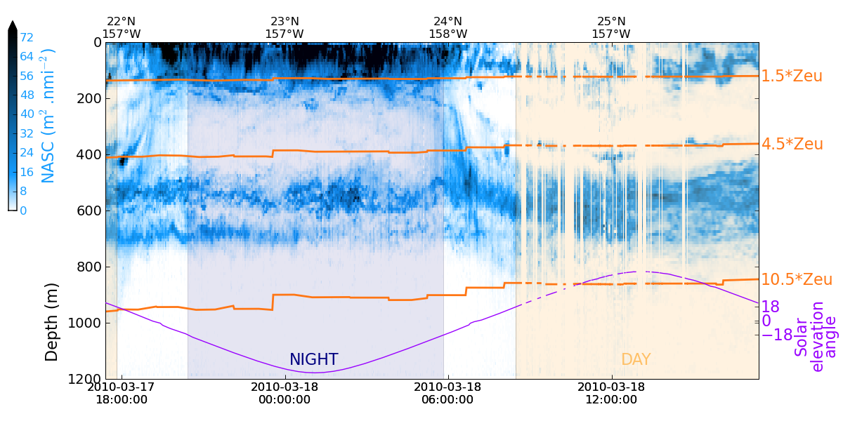
Figure 1: Example of a portion of acoustic transect. After the vertical layers have been defined the signal strength is vertically integrated and then averaged at the spatial resolution of the grid of the model (1/4°) after excluding the sunset and sunrise time periods. The orange lines delineate the vertical layers boundaries based on the euphotic depth. The purple line shows the variation of the solar elevation angle (which is used to discriminate between night and day) through the day, from Lehodey & al. (submitted)
WP4000: Prototype demonstration and impact assessmentWP4000: Prototype demonstration and impact assessment
The prototype products will be generated depending of the outcome of the WP1200 which will define in particular the period and area of interest for the applications.
WP4100 Production of experimental datasets
WP 4110 surface salinity fields
A prototype production chain for the merged in-situ-satellite SSS L4 product will be developed and implemented at the CNR computing facility in Rome, based on the pre-existing scientific software developed by CNR in the framework of a Myocean R&D project (MESCLA project) and the results of WP3100. The time series of level 4 SSS product (covering the test period and area selected) will thus be produced by CNR on its own computing facilities. The prototype chain will be set-up taking advantage of the experience gained by CNR in the framework of Myocean-2 OCTAC and OSITAC.
WP 4120 Production of 3D ocean state fields
A prototype production chain for the estimation of the 3D ocean temperature, salinity and currents from the combined use of GOCE data, altimetry, satellite SSS and SST data, in-situ data, will be developed and implemented at CLS based on the pre-existing software developed in the framework of previous projects (Mersea, MyOcean).
WP4130 Project Dataset update
In this task, the Project Dataset and corresponding Dataset User Manual initiated in WP2000 will be updated to include the new experimental datasets produced in WP4110 and 4120. Both datasets and Data User Manual will be put on the project website and made freely available for public use.
WP4200 Demonstration
In this task the experimental datasets (net primary production, euphotic layer depth, temperature, ocean currents) produced in WP4100 will be used as inputs to the micronekton model in order to estimate a time series of the different functional micronekton groups biomasses distribution.
WP 4300 Impact assessment
In this task, the
benefit and impact of developed products/methods
on the specific test areas will be assessed. In order to carefully
analyze the errors/uncertainties on the micronekton density maps, a
comparison of the model outputs to in-situ acoustic measurements of the
micronekton will be done. This will be done in close collaboration with
colleagues expert in acoustic data analyses.
Also, in order to better assess the potential benefit and impact of the
study on the scientific and operational production of micronekton maps,
a comparison will be done with a global reanalysis of micronekton
density that has been recently produced at CLS using outputs from the
Mercator-Ocean model for the physical forcing of the model.
This workpackage will be done with the support of different partners
with which CLS has already a strong collaboration on this topic. Two
types of partners will be involved, those specialist of the in-situ
acoustic measurements of micronekton, that will be able to help
evaluate the micronekton model outputs in their area of interest, and
those involved in the management of marine resources and potentially
interested by the development of new applications from these products:
- The CSIRO (Commonwealth Scientific and Industrial Research
Organisation) Marine and Atmospheric Research (CMAR)
The CMAR contributes to the development of acoustic/sound methods to sample and study the components of macroplankton and micronekton of the ocean ecosystem in the context of sustainable fisheries management. - The Pacific Islands Fisheries Science Center (PIFSC), the
National Marine Fisheries Service (NMFS) from the US National Oceanic
and Atmospheric Organization (NOAA)
The NMFS of the National Oceanic and Atmospheric Administration (NOAA) is the federal agency responsible for the management, conservation and protection of living marine resources in the Exclusive Economic Zone of the United States. The PIFSC is one of the regional offices. Its goal is to promote sustainable fisheries and prevent economic loss related to potentially abusive fisheries, endangered species and habitat degradation NMFS goal. - The Biological Study Center of Chiza, CNRS, France.
- The Biological Study Center of Chiza (CEBC), CNRS, France
The CEBC is one of the leading center on marine mammals and marine birds ecology since several decades. The team is internationally recognized for its numerous studies on large marine predators demography and ecology and the impact of the environmental variability on these animal populations. - Secretariat of the Pacific Community (CPS) ), Oceanic Fishing
Program (OFP), Nouvelle-Caledonie
The OFP contributes to the objectives of the CPS to implement the vision of the regional policy of the Pacific Islands: "A healthy ocean that supports life and aspirations of Pacific Island communities." The OFP provides scientific services relating to the management of ocean fisheries (mainly tuna) and its members directly to the Fisheries Commission and Central Pacific Ocean (WCPFC). These services include fisheries monitoring and management of data, research on the biology and ecosystems associated with fisheries, stock assessment, and evaluation of management scenarios based on species and ecosystems. - The National Research Institute of Far Seas Fisheries (NRIFSF)
The NRIFSF was founded in 1967. This is one of the institutes of the Agency for Fisheries Research of Japan, whose research focuses on tuna, whales and dolphins, squid, groundfish worldwide and krill in the Antarctica. NRIFSF objectives are to contribute to the rational use of renewable resources through scientific information obtained by its research resources. Some of its activities are conducted in collaboration with domestic and foreign organizations and international organizations.
Output:
An Impact Assessment Report (IAR) will be prepared that will collect
the final findings and results of this Impact Assessment activity.
WP5000: Scientific Roadmap
Building on the outputs of the different tasks listed above, a Scientific Roadmap will be defined in this task, in order to best prepare the transfer of the outcomes of the project into future scientific and operational activities.
Output:
The following outputs will be delivered as required:
Scientific Roadmap (SR) document that will define strategic actions for
fostering a transition of the target methods and model developed in the
project from research to operational activities.
WP6000: Promotion
Technical
description:
As required in the SoW, the promotion workpackage will comprise the
following activities:
- Creation and maintenance of a dedicated project website
A project website will be developed for communicating to the general public and the scientific community the objectives and main outcomes of the project. The website will also provide a direct access to the different prototype products and experimental datasets developed during the project. In addition, it will include an internal webpage (password protected accessible for ESA and consortium members) for supporting management and documentary activities. The project web page content will be maintained and updated at least every month to include updated deliverable items and content for the duration of the contract. - Participation to Relevant Scientific Events
The contractor will prepare a list of scientific events/ workshops occurring during the life of the project that are relevant to the promotion of the project activities.
The contractor will prepare material (poster or viewgraphs) to be used for these occasions. - Contribution to scientific literature
One or more scientific publications will be submitted in peer-reviewed journals with the findings and novelties of this project.
Output:
The following outputs will be delivered as required:
- project website,
- publications
- presentations
WP7000: Management and Reporting
Technical
description
In this work-package, the Prime will coordinate the work done in the
different work packages.
The management and reporting work will include: project administration,
contractual negotiation, contract administration, organisation and
participation to meetings, project/financial/resources control,
planning and schedule control, preparation of meetings, of minutes and
maintenance of action item lists after each meeting. In addition, a
number of reports will be issued including monthly progress reports, a
final report for public access and an executive summary of the project
summarizing relevant achievements.
All the management work will be summarized in a formal living document
called Project Management Plan that recalls the project scope and
work package content, that updates the Working Plan and scheduling
(according a Work Breakdown Structure Graph and a Gantt Chart), list of
deliverables and planned delivery dates and proposed Table of Contents
for the deliverables.
Output:
The prime will issue monthly
reports and send them to ESA with the
updated progress report and completion schedule of the different work
packages in the last month, the list of the issues encountered and
proposed corrective solutions, the status of the minute action items,
and the list of submitted and to be submitted deliveries.
The Prime of the contract will
deliver to ESA the deliverables of the
different Work Packages, the project management plan, the minutes of
the progress meetings, the final report and the Executive Summary.